RUNNING
EQS
|
|
Double
click on the "EQS for Windows" icon and the following window appears:
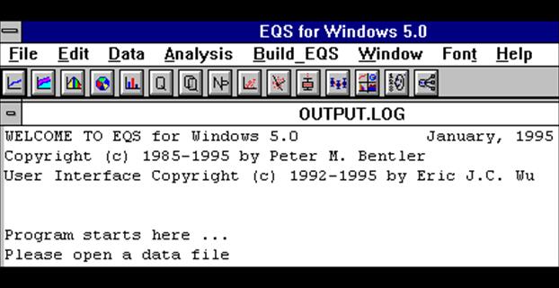
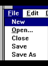
Click on
File and the next window appears:
EQS Rules,
Definitions and Operations
Merle
Canfield
The
block diagrams can be used first to create a model or theory. That diagram can then be used to create the
equations for testing the model. The
block diagram then represents the structural model to be tested. The following are rules for drawing the block
diagrams.
1. Variables in the input data file to
be analyzed are observed or measured variables; called Vs in EQS (p 13). They are represented by rectangles in the
block diagram.
2. Hypothetical constructs are
unmeasured latent variables, as in factor analysis, and are called factors or
Fs (p 13). They are represented by
circles in the block diagram.
3. Residual variation in measured
variables is generated by errors or Es (p 13).
Represented by E on the block diagram.
4. Residual variation of unmeasured
(latent) variables is generated by errors in the equations are called Ds or
disturbances in EQS (p 18). Represented
by D on the block diagram.
5. A straight arrow with a single
pointer represents casual or directional influence of one variable (either
measured or latent) on another (p. 17).
6. An arrow with dual pointers (the
arrow can be either curved or straight) represents a correlation or covariation
between two variables (it is sometimes not curved -- the dual pointers
determine it's nature) (p. 17). These
represent regression coefficients.
7. All arrows represent parameters of
the equation.
8. Arrows that have asterisks indicate
that the parameter is to be estimated.
9. Arrows that have a "1"
indicate that the parameter is set to be 1.
10. Arrows that have a "0"
indicate that the parameter is set to be 0.
11. Arrows that have no symbols indicate
that the parameter is set to be 1.
12. An absence of arrows between two
elements (error or variables) indicates that the path is set to 0.
13. EQS cannot deal with dependent
categorical variables (p 5).
14. The ratio of sample size to number of
free parameters to be estimated may be able to go as low as 5:1 under normal
and elliptical theory (p 6).
15. There is one equation for each
dependent variable in the system (p 7).
16. A dependent variable is one that is a
structured regression function of other variables; it is recognized in a path
diagram by having one or more arrows aiming at it (p 7).
17. Every independent variable in the
model must have a variance (p 7).
18. Dependent variables cannot have
variances or covariances with other variables as parameters of a structural
model (p 16).
19. df = measured variables * (measured
variables + 1)/2 (p 18).
20. Every unmeasured variable (i.e. F, E,
and D variables) in a structural model must have its scale determined. This can always be done by fixing a path from
that variable to another variable at some known value (usually 1.0). An alternative method for determining the
scale of an independent unmeasured variable is to fix its variance at some
known value (usually 1.0) (p 18).
21. When the V999 variable is used a
/MEANS command is required (p. 168).
22. When using the error variance of a
variable or a factor to assess the variance accounted for and test such
variance with a chi square change by removing an arrow this can be done only
with an arrow pointing at the variable being assessed. The arrow removed must be the only change in
the model.
23. Except for special cases a factor must
have at least two variables.
RUNNING
EQS
|
|
Double
click on the "EQS for Windows" icon and the following window appears:
Click on
File and the next window appears:
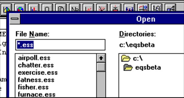
Click on
Open and the next window appears:
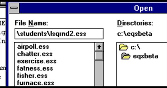
Type
"\students\lsqrnd2.ess" in the File Name box so that it looks like
this:
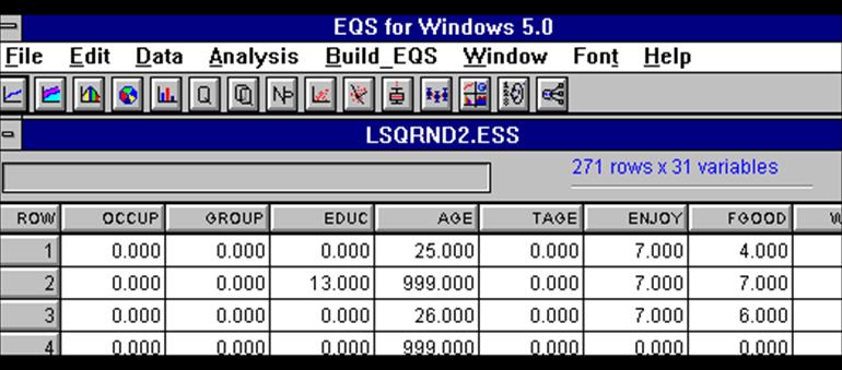
Click OK
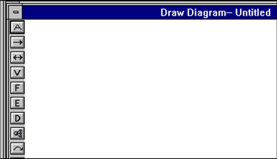
or press return and the following window appears:
Click on
the last button of the "button bar" or "power bar" (it is
just below the last 'w' of Window) and the next screen will appear:
Click on
the button below the "D" (it is similar to the previous button
selected). Move the + to the left side
of the "drawing area." The
following window will appear:
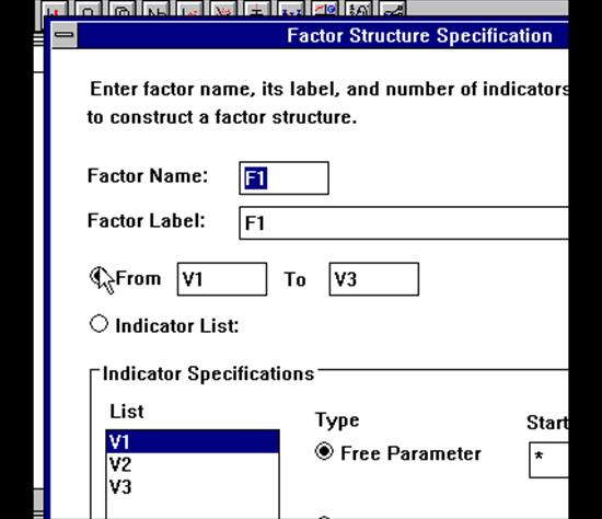
It
should be filled in like the next box:
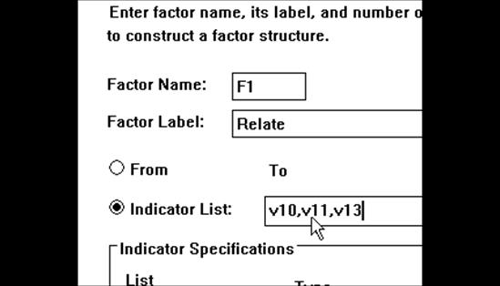
And then
click Apply; click OK. The following
graph will appear:
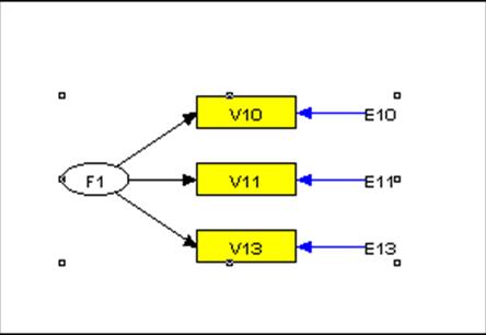
It is
turned the wrong direction.
Click
Edit;click Select All
Click
Edit; click Horizontal Flip
Click
the "cat paw" again (the button just below the "D"):
Move the
+ to the right side of the drawing area and click:
File in
the window like this:
Click
Apply;
click OK
Click
Edit; click Select All
Click
Edit; click Align Horizontal
Click on
"right arrow" button: move + to just inside the right side of the F1
circle and click
move + to just inside the left side of the F2 circle and click
Click
View
Click
Labels
The
drawing should look like this:

Click
File
Click
Save As
File in
the window as follows:
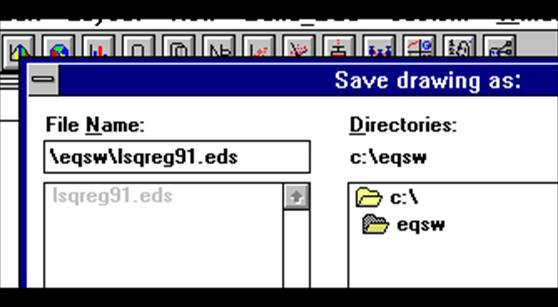
Click
OK; click "Yes"
Click
Build_EQS; click Title/Specifications
File in
the window as follows:
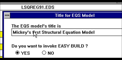
Click OK
Click OK
to the next window and the following jobstream appears:
save it
Click on
Build_EQS
Click on
Run EQS/386
Click OK
Save
File
Select
Diagram
Click
View
Select
Estimates
Select
Standardized Solution
The
diagram should look like this.