Cluster
Analysis
Merle
Canfield
The
purpose of cluster analysis is to categorize a set of objects, variables, or
people by placing them into clusters based on their similarity or
differences. It is a method for
developing a taxonomy. If variables are
clustered then it is like factor analysis although there are differences that
will be demonstrated below. In fact, a
correlation may used in cluster analysis.
The
questionnaire on the next page is used in this cluster analysis example. Like discriminant function, cluster analysis
is a method of grouping individuals, or variables. In the first example individuals are
clustered and in the second example variables are clustered. The same set of data is used in both
examples.
The
difference between discriminant function and cluster analysis is that
discriminant function the groups are known and the task is to identify the
variables that will predict which group the individual should be assigned to,
while in cluster analysis the groups are empirically derived from the
variables.
SETTING QUESTIONNAIRE
NAME
________________________________________
DATE ___________________
SETTING
_____________________________________
TIME ___________________
INSTRUCTIONS: For each item draw a circle around the number
that you
think best describes the
setting. IMPORTANT: If you think
that some people are acting or
feeling one way and other
people are acting or feeling
another way then both may be
circled. Two numbers may be circled for one item. Do not
circle more than two. Try hard to circle only one.
When people are in this setting they are:
seldom often
1. 0
1 2 3 4 5 6 7 8 tense
2. 0
1 2 3 4 5 6 7 8 satisfied
3. 0
1 2 3 4 5 6 7 8 easy going
4. 0
1 2 3 4 5 6 7 8 caring
5. 0
1 2 3 4 5 6 7 8 good
6. 0
1 2 3 4 5 6 7 8 friendly
7. 0
1 2 3 4 5 6 7 8 confident
8. 0
1 2 3 4 5 6 7 8 suspicious
9. 0
1 2 3 4 5 6 7 8 lazy
10. 0 1 2 3 4 5 6 7 8 forced to do things
11. 0 1 2 3 4 5 6 7 8 busy
12. 0 1 2 3 4 5 6 7 8 ordered around
When people are in this setting they:
13. 0 1 2 3 4 5 6 7 8 have a say about what to do
14. 0 1 2 3 4 5 6 7 8 share
15. 0 1 2 3 4 5 6 7 8 know what's going on
16. 0 1 2 3 4 5 6 7 8 think
17. 0 1 2 3 4 5 6 7 8 work together
18. 0 1 2 3 4 5 6 7 8 have high self‑esteem
19. 0 1 2 3 4 5 6 7 8 learn
20. 0 1 2 3 4 5 6 7 8 joke around
21. 0 1 2 3 4 5 6 7 8 can come and go as they want
22. 0 1 2 3 4 5 6 7 8 talk about personal problems
23. 0 1 2 3 4 5 6 7 8 have a good time
In this setting:
24. 0 1 2 3 4 5 6 7 8 things get done
25. 0 1 2 3 4 5 6 7 8 its easy to fit in
26. 0 1 2 3 4 5 6 7 8 there is conflict
27. 0 1 2 3 4 5 6 7 8 people like each other
|
File
Name = psscls1.sps
|
|
get file="E:\rdda\pssstf16.sav".
CLUSTER tense
satisfie easygoin caring good friendly confiden suspicio lazy
forced busy
ordered whattodo share goingon think worktoge selfeste learn
joke comeandg
personal goodtime thingsge easyfiti conflict peopleli
/METHOD BAVERAGE
/MEASURE= SEUCLID
/ID=personra
/PRINT SCHEDULE
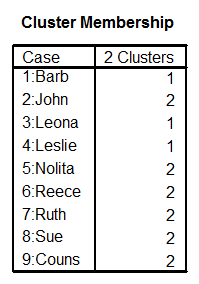
CLUSTER(2)
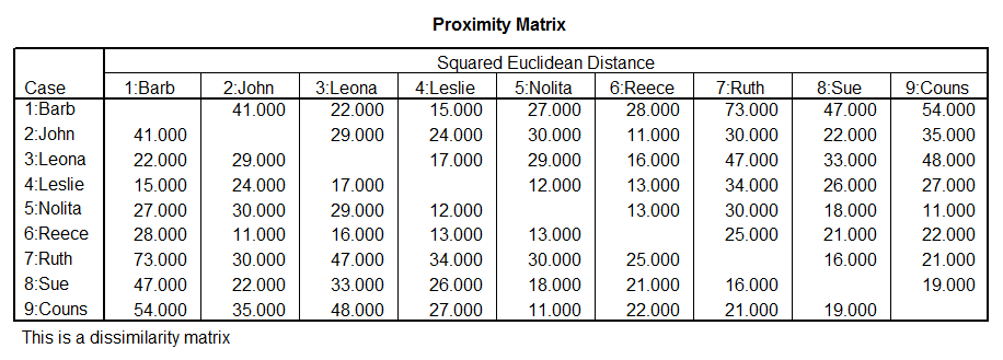
/PRINT DISTANCE
/PLOT DENDROGRAM
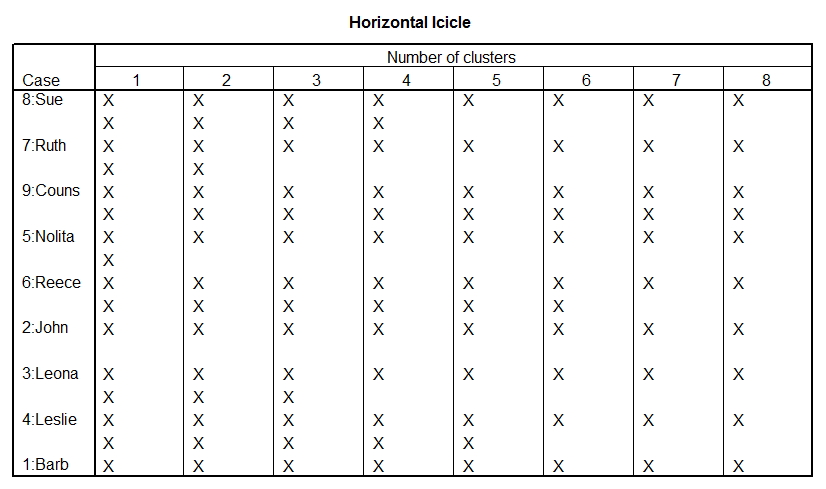
HICICLE.
|
The
above file was generated with the following clicks:
Click
Analyze
Click
Classify
Click
Hierarchical Cluster
Select
ID
Click
right delta for Label Cases By:
Select
Variables to use for clustering
Click
right delta for Variables
Click
Statistics
Select
Agglomeration
Select
Proximity Matrix
Select
Single Solution and 2 clusters
Click
Continue
Click
Plots
Select
Dendrogram
Select
Horizontal
Click
Continue
Click
Method
Click
OK
|
PERSONRA
|
TENSE
|
SATISFIED
|
EASYGOING
|
CARING
|
GOOD
|
FRIENDLY
|
CONFIDENT
|
SUSPICIOUS
|
LAZY
|
FORCED
|
BUSY
|
ORDERED
|
WHATTODO
|
SHARE
|
GOINGON
|
THINK
|
WORKTOGETH
|
SELFESTEEM
|
LEARN
|
JOKE
|
COMEANDGO
|
PERSONAL
|
GOODTIME
|
THINGSGET
|
EASYFITIN
|
CONFLICT
|
PEOPLELIKE
|
|
Barb
|
2
|
6
|
6
|
8
|
6
|
7
|
6
|
1
|
2
|
2
|
5
|
1
|
7
|
7
|
7
|
6
|
7
|
7
|
6
|
6
|
5
|
4
|
6
|
6
|
7
|
3
|
6
|
|
John
|
4
|
5
|
4
|
6
|
6
|
6
|
5
|
2
|
2
|
2
|
5
|
2
|
5
|
6
|
6
|
7
|
6
|
6
|
7
|
4
|
5
|
4
|
4
|
5
|
5
|
2
|
6
|
|
Leona
|
2
|
5
|
5
|
7
|
6
|
7
|
6
|
1
|
1
|
1
|
6
|
2
|
6
|
6
|
7
|
7
|
6
|
6
|
7
|
5
|
5
|
4
|
4
|
6
|
7
|
5
|
6
|
|
Leslie
|
3
|
5
|
5
|
7
|
5
|
6
|
6
|
2
|
2
|
2
|
5
|
2
|
6
|
6
|
7
|
6
|
6
|
6
|
6
|
6
|
5
|
5
|
6
|
6
|
6
|
4
|
6
|
|
Nolita
|
3
|
5
|
5
|
7
|
6
|
7
|
6
|
2
|
3
|
3
|
5
|
3
|
6
|
6
|
6
|
5
|
6
|
6
|
5
|
5
|
4
|
6
|
5
|
6
|
6
|
4
|
6
|
|
Reece
|
3
|
5
|
5
|
6
|
6
|
6
|
5
|
2
|
2
|
2
|
5
|
2
|
6
|
6
|
6
|
6
|
6
|
6
|
6
|
4
|
5
|
5
|
4
|
5
|
6
|
4
|
6
|
|
Ruth
|
4
|
5
|
4
|
5
|
5
|
5
|
6
|
3
|
2
|
3
|
6
|
4
|
5
|
6
|
6
|
6
|
6
|
5
|
5
|
4
|
4
|
4
|
4
|
6
|
4
|
5
|
5
|
|
Sue
|
4
|
5
|
4
|
7
|
6
|
6
|
6
|
2
|
2
|
4
|
6
|
3
|
5
|
6
|
6
|
6
|
6
|
6
|
6
|
4
|
3
|
4
|
4
|
7
|
5
|
4
|
6
|
|
Couns
|
4
|
5
|
5
|
7
|
6
|
6
|
6
|
2
|
2
|
4
|
5
|
4
|
5
|
6
|
6
|
5
|
6
|
5
|
4
|
5
|
4
|
6
|
4
|
5
|
5
|
4
|
6
|
Cluster
Average Linkage (Between
Groups)
Dendrogram
_
* * * * * * H I E R A R C H I C A L C L U S T E R A N A L Y S I S * * * * * *
Dendrogram using Average Linkage (Between
Groups)
Rescaled
Distance Cluster Combine
C A S E 0 5 10 15 20 25
Label Num
+---------+---------+---------+---------+---------+
Nolita 5
òûòòòòòòòòòòòòòòòòòòòòòòòø
Couns 9 ò÷ ùòòòòòø
Ruth 7 òòòòòòòòòòòûòòòòòòòòòòòòò÷ ùòòòòòòòòòòòòòòòòòø
Sue 8 òòòòòòòòòòò÷ ó ó
John 2 òûòòòòòòòòòòòòòòòòòòòòòòòòòòòòò÷ ó
Reece 6 ò÷ ó
Barb 1 òòòòòòòòòûòòòòòòòòòø
ó
Leslie 4
òòòòòòòòò÷ ùòòòòòòòòòòòòòòòòòòòòòòòòòòòòò÷
Leona 3 òòòòòòòòòòòòòòòòòòò÷
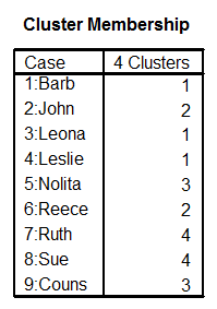
The
next analysis request four clusters.
|
File
Name = psscls2.sps
|
|
get
file = '\rdda\pssstf16.sav'.
cluster
tense to peoplelia
/id=personra
/print=distance
/print=schedule cluster(4)
/plot=dendrogram hicicle.
|
Cluster
>Warning # 708 in column 18. Text: PEOPLELIA
>A variable name is more than 8 characters
long. Only the first 8
>characters will be used.
Average Linkage (Between
Groups)
Dendrogram
_
* * * * * * H I E R A R C H
I C A L C L U S T E R A N A L Y S I S * * * * * *
Dendrogram using Average Linkage (Between
Groups)
Rescaled
Distance Cluster Combine
C A S E 0 5 10 15 20
25
Label Num
+---------+---------+---------+---------+---------+
Nolita 5
òûòòòòòòòòòòòòòòòòòòòòòòòø
Couns 9 ò÷ ùòòòòòø
Ruth 7 òòòòòòòòòòòûòòòòòòòòòòòòò÷ ùòòòòòòòòòòòòòòòòòø
Sue 8 òòòòòòòòòòò÷ ó ó
John 2 òûòòòòòòòòòòòòòòòòòòòòòòòòòòòòò÷ ó
Reece 6 ò÷ ó
Barb 1 òòòòòòòòòûòòòòòòòòòø
ó
Leslie 4
òòòòòòòòò÷ ùòòòòòòòòòòòòòòòòòòòòòòòòòòòòò÷
Leona 3 òòòòòòòòòòòòòòòòòòò÷
Transposing
a File
Click
on Data; Click on Transpose; Click on PERSONA; Click on delta to Variable Name;
Select remaining variables; Click on delta to Variables; Click OK. SAVE AS pssstf18.sav.
|
ITEM
|
BARBE
|
JOHN
|
LEONA
|
LESLIE
|
NOLITA
|
REECE
|
RUTH
|
SUE
|
COUNS
|
|
TENSE
|
2
|
4
|
2
|
3
|
3
|
3
|
4
|
4
|
4
|
|
SATIS
|
6
|
5
|
5
|
5
|
5
|
5
|
5
|
5
|
5
|
|
EASY
|
6
|
4
|
5
|
5
|
5
|
5
|
4
|
4
|
5
|
|
CARE
|
8
|
6
|
7
|
7
|
7
|
6
|
5
|
7
|
7
|
|
GOOD
|
6
|
6
|
6
|
5
|
6
|
6
|
5
|
6
|
6
|
|
FRIEND
|
7
|
6
|
7
|
6
|
7
|
6
|
5
|
6
|
6
|
|
CONFI
|
6
|
5
|
6
|
6
|
6
|
5
|
6
|
6
|
6
|
|
SUSP
|
1
|
2
|
1
|
2
|
2
|
2
|
3
|
2
|
2
|
|
LAZY
|
2
|
2
|
1
|
2
|
3
|
2
|
2
|
2
|
2
|
|
FORCED
|
2
|
2
|
1
|
2
|
3
|
2
|
3
|
4
|
4
|
|
BUSY
|
5
|
5
|
6
|
5
|
5
|
5
|
6
|
6
|
5
|
|
ORDER
|
1
|
2
|
2
|
2
|
3
|
2
|
4
|
3
|
4
|
|
WHATDO
|
7
|
5
|
6
|
6
|
6
|
6
|
5
|
5
|
5
|
|
SHARE
|
7
|
6
|
6
|
6
|
6
|
6
|
6
|
6
|
6
|
|
GOON
|
7
|
6
|
7
|
7
|
6
|
6
|
6
|
6
|
6
|
|
THINK
|
6
|
7
|
7
|
6
|
5
|
6
|
6
|
6
|
5
|
|
WORKT
|
7
|
6
|
6
|
6
|
6
|
6
|
6
|
6
|
6
|
|
SELFE
|
7
|
6
|
6
|
6
|
6
|
6
|
5
|
6
|
5
|
|
LEARN
|
6
|
7
|
7
|
6
|
5
|
6
|
5
|
6
|
4
|
|
JOKE
|
6
|
4
|
5
|
6
|
5
|
4
|
4
|
4
|
5
|
|
COMEGO
|
5
|
5
|
5
|
5
|
4
|
5
|
4
|
3
|
4
|
|
PERSONAL
|
4
|
4
|
4
|
5
|
6
|
5
|
4
|
4
|
6
|
|
TOODT
|
6
|
4
|
4
|
6
|
5
|
4
|
4
|
4
|
4
|
|
THINGSD
|
6
|
5
|
6
|
6
|
6
|
5
|
6
|
7
|
5
|
|
EASYF
|
7
|
5
|
7
|
6
|
6
|
6
|
4
|
5
|
5
|
|
CONFLCT
|
3
|
2
|
5
|
4
|
4
|
4
|
5
|
4
|
4
|
|
PEOPLL
|
6
|
6
|
6
|
6
|
6
|
6
|
5
|
6
|
6
|
|
File
Name = psscls3.sps
|
|
get
file = '\rdda\pssstf18.sav'.
cluster
barb to couns
/id=case_lbl
/print=distance
/print=schedule cluster(3)
/plot=dendrogram hicicle.
|
Cluster
>Warning # 708 in column 18. Text: PEOPLELIA
>A variable name is more than 8 characters
long. Only the first 8
>characters will be used.
Average Linkage (Between
Groups)
Dendrogram
_
* * * * * * H I E R A R C H I C A L C L U S T E R A N A L Y S I S * * * * * *
Dendrogram using Average Linkage (Between
Groups)
Rescaled Distance
Cluster Combine
C
A S E 0 5 10 15 20 25
Label Num
+---------+---------+---------+---------+---------+
Nolita 5 òûòòòòòòòòòòòòòòòòòòòòòòòø
Couns 9 ò÷ ùòòòòòø
Ruth 7 òòòòòòòòòòòûòòòòòòòòòòòòò÷ ùòòòòòòòòòòòòòòòòòø
Sue 8 òòòòòòòòòòò÷ ó ó
John 2 òûòòòòòòòòòòòòòòòòòòòòòòòòòòòòò÷ ó
Reece 6 ò÷ ó
Barb 1 òòòòòòòòòûòòòòòòòòòø ó
Leslie 4 òòòòòòòòò÷ ùòòòòòòòòòòòòòòòòòòòòòòòòòòòòò÷
Leona 3 òòòòòòòòòòòòòòòòòòò÷
Cluster
Average Linkage (Between
Groups)
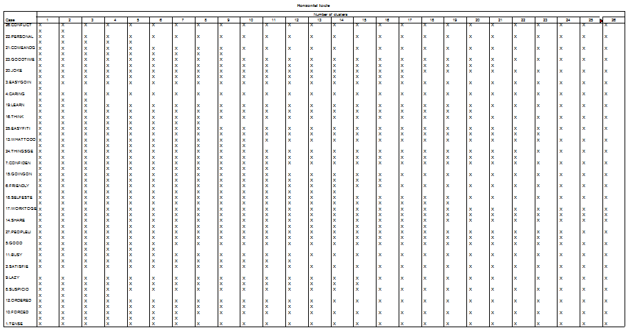
Dendrogram
Dendrogram using Average Linkage (Between
Groups)
Rescaled Distance
Cluster Combine
C A S
E 0 5 10 15 20 25
Label Num
+---------+---------+---------+---------+---------+
SHARE 14 òø
WORKTOGE 17 òú
SELFESTE 18 òú
GOOD 5 òôòø
PEOPLELI 27 òú ó
FRIENDLY 6 òú ó
GOINGON 15 ò÷ ó
CONFIDEN 7 òûò÷
THINGSGE 24 ò÷ ó
WHATTODO 13 òûòüòø
EASYFITI 25 ò÷ ó ó
THINK 16 òûò÷ ùòø
LEARN 19 ò÷ ó ó
SATISFIE 2 òûòòò÷ ùòòòòòø
BUSY 11 ò÷ ó ó
CARING 4 òòòòòòò÷ ó
JOKE 20 òø
ùòòòòòòòòòòòòòòòòòòòòòòòòòòòòòòòòòòòø
GOODTIME 23 òôòø ó
ó
EASYGOIN 3 ò÷ ùòø ó
ó
COMEANDG 21 òòò÷ ùòòòø ó
ó
PERSONAL 22 òòòòò÷ ùòòò÷
ó
CONFLICT 26 òòòòòòòòò÷ ó
SUSPICIO 8 òûòòòòòø ó
LAZY 9 ò÷ ùòòòòòòòòòòòòòòòòòòòòòòòòòòòòòòòòòòòòòòòòò÷
FORCED 10 òûòø ó
ORDERED 12 ò÷ ùòòò÷
TENSE 1 òòò÷
The purpose of this section is to show the relationships
among correlation and cluster analysis.
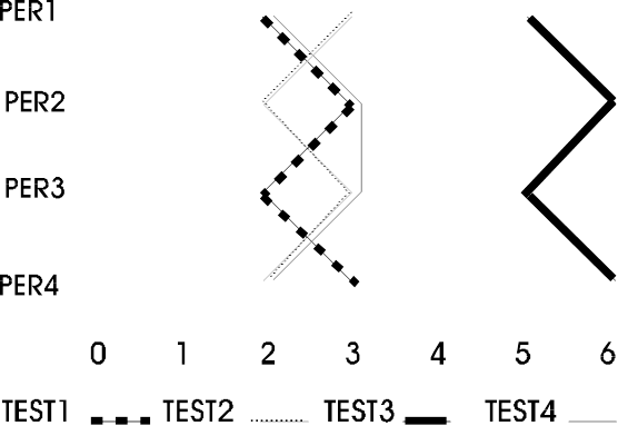
In this example 4 people have taken 4 tests (tests are like
variables). The data are as follows:
The purpose of this next section
is twofold: (1) to demonstrate another method of the use of the statistics and
(2) compare the various statistics methodologically.
The purpose of this section is to
show the relationships between correlation (and factor analysis), and cluster
analysis. In this example 4 people have
taken 4 tests (tests are like variables).
The data are as follows:
|
CLSDAT1.TXT
|
|
"PER1",2,3,5,2
"PER2",3,2,6,3
"PER3",2,3,5,3
"PER4",3,2,6,2
|
The
data is presented graphically:
[COMMENT1]
Correlation of variables (and
consequently factor analysis) will indicate the similarity of tests in terms of
their relative position of each individual on the test, while cluster
analysis will indicate the similarity of tests using the absolute
position difference of each individual on the test. The correlation is presented:
|
File Name = crscor16.sps
|
|
get file = '\proeval\CLSDAT1.sav'
/keep= PERs TEST1 TEST2 TEST3 TEST4.
COR TEST1 TO TEST4
/STATISTICS=all.
|
Correlations
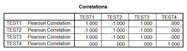
In Frame CRSCOR16.LIS TEST1,
TEST2, and TEST3 all correlate perfectly with each other, even though test 2 is
negatively correlated with the other two.
Test4 correlates zero with all three tests. It can be seen in the graphic that the
profiles of TEST1 and TEST3 are identical even though are separated in terms of
distance. TEST2 is the mirror image of
the other two. TEST4 although close in
proximal distance to TEST1 and TEST2 is quite dissimilar in terms of the
relative shape or profile.
Factor analysis shows how this
small set of variable can be summarized.
It should be noted that there are not nearly enough variables in this
set for what would be considered appropriate; there should be at a minimum 40
subjects to compute this analysis. The
purpose of this example is to show the differential effects of factor analysis
and cluster analysis. As indicated the
two analysis are similar in that they both summarize the possible underlying
characteristics of a set of variables thus simplifying and consequently
obtaining more parsimony. However, the
summarization process is somewhat different for the two processes and this
demonstration is designed to show.
|
File Name = crsfac8.sps
|
|
get file =
'\proeval\CLSDAT1.sav'
/keep= PERs TEST1 TEST2 TEST3 TEST4.
fac var= test1 to test4
/ rotation.
|
┌───────────────────────────────────────────────────────────────────────────┐
│ CRSFAC8.SPS │
├───────────────────────────────────────────────────────────────────────────┤
│Final Statistics: │
│
│
│Variable Communality *
Factor Eigenvalue Pct of Var
Cum Pct │
│ * │
│TEST1 1.00000 *
1 3.00000 75.0 75.0
│
│TEST2 1.00000 *
2 1.00000 25.0 100.0
│
│TEST3 1.00000 * │
│TEST4 1.00000 *
│
│
│
│Varimax Rotation
1, Extraction 1,
Analysis 1 ‑ Kaiser
Normalization.│
│ │
│ Varimax converged in 2 iterations. │
│
│
│Rotated Factor
Matrix: │
│
│
│ FACTOR 1
FACTOR 2 │
│
│
│TEST1 1.00000 .00000 │
│TEST2 ‑1.00000 .00000 │
│TEST3 1.00000 .00000 │
│TEST4 .00000 1.00000 │
└───────────────────────────────────────────────────────────────────────────┘
TEST1,
TEST2, and TEST3 form the first factor and TEST4 forms a factor of its
own. Further, the first three variables
are perfectly correlated with the first factor.
However, TEST2 is negatively correlated with the factor. The relative weights are perfectly related.
The
cluster analysis is presented. It is
necessary to invert the data in order for the analyses to be comparable as
shown in Frame CLSDAT2.TXT. Frame
CRSCLS7.SPS contains the jobstream and Frame CRSCLS7.LIS contains the output.
|
CLSDAT2.sav
|
|
"TEST1",2,3,2,3
"TEST2",3,2,3,2
"TEST3",5,6,5,6
"TEST4",2,3,3,2
|
|
File
Name = crscls7.sps
|
|
get
file = '\proeval\CLSDAT2.sav'
/keep= ID
PER1 PER2 PER3 PER4.
cluster
PER1 TO PER4
/id=ID
/print=distance
/print=schedule cluster(2)
/plot=dendrogram hicicle.
|
┌───────────────────────────────────────────────────────────────────────────┐
│ CRSCLS7.LIS │
├───────────────────────────────────────────────────────────────────────────┤
│ Squared Euclidean measure
used.
│
│
│
│ 1 Agglomeration
method specified. │
│ │
│ Squared Euclidean
Dissimilarity Coefficient Matrix │
│
│
│ Case 1 2 3 │
│
│
│ 2 4.0000
│
│ 3
36.0000 40.0000 │
│ 4 2.0000 2.0000 38.0000 │
│
│
│
│
│ Number of
Clusters │
│
│
│ Label
Case 2
│
│
│
│ TEST1
1 1
│
│ TEST2
2 1
│
│ TEST3
3 2
│
│ TEST4
4 1
│
│
│
│
│
│ │
│ Dendrogram using
Average Linkage (Between Groups) │
│
│
│ Rescaled Distance
Cluster Combine │
│
│
│ C A S E 0
5 10 15 20 25
│
│ Label
Seq +‑‑‑‑‑‑‑‑‑+‑‑‑‑‑‑‑‑‑+‑‑‑‑‑‑‑‑‑+‑‑‑‑‑‑‑‑‑+‑‑‑‑‑‑‑‑‑+ │
│
│
│ TEST2
2 ‑+
│
│ TEST4
4 ‑+‑‑‑‑‑‑‑‑‑‑‑‑‑‑‑‑‑‑‑‑‑‑‑‑‑‑‑‑‑‑‑‑‑‑‑‑‑‑‑‑‑‑‑‑‑‑‑+ │
│ TEST1
1 ‑+
| │
│ TEST3
3 ‑‑‑‑‑‑‑‑‑‑‑‑‑‑‑‑‑‑‑‑‑‑‑‑‑‑‑‑‑‑‑‑‑‑‑‑‑‑‑‑‑‑‑‑‑‑‑‑‑+ │
└───────────────────────────────────────────────────────────────────────────┘
Note
in the cluster analysis that there are also two clusters representing the four
variables but they are constructed of different variables or tests than the
factor analysis. TEST1, TEST2, and TEST4
make up cluster1 and TEST3 is in a cluster alone. The calculations below show that in the
correlation (factor analysis) a relative relationship among variables and
cluster analysis assesses an absolute relationship.
A
more detailed inspection of the analysis will demonstrate the differences. The following jobstream and output shows how
the correlation and factor analysis operate in relative terms.
|
File
Name = crslis1.sps
|
|
get
file = '\proeval\CLSDAT1.sav'
/keep= PERs TEST1 TEST2 TEST3 TEST4.
COMPUTE
T1LX = TEST1 ‑ 2.5.
COMPUTE
T2LX = TEST2 ‑ 2.5.
COMPUTE
T3LX = TEST3 ‑ 5.5.
COMPUTE
T4LX = TEST4 ‑ 2.5.
COMPUTE
T1LX2=T1LX*T1LX.
COMPUTE
T2LX2=T2LX*T2LX.
COMPUTE
T3LX2=T3LX*T3LX.
COMPUTE
T4LX2=T4LX*T3LX.
COMPUTE
T1LXT2LY=T1LX*T2LX.
COMPUTE
T1LXT3LY=T1LX*T3LX.
COMPUTE
T1LXT4LY=T1LX*T4LX.
LIST
T1LX T2LX T3LX T4LX .
LIST
T1LX2 T2LX2 T3LX2 T4LX2 T1LXT2LY T1LXT3LY T1LXT4LY.
|
|
CRSLIS1.LIS
|
|
T1LX T2LX
T3LX T4LX
‑.50 .50
‑.50 ‑.50
.50
‑.50 .50 .50 ‑.50 .50
‑.50 .50 .50 ‑.50 .50
‑.50
T1LX2 T2LX2
T3LX2 T4LX2 T1LXT2LY T1LXT3LY
T1LXT4LY .25 .25
.25 .25 ‑.25 .25
.25 .25 .25
.25 .25 ‑.25 .25
.25 .25 .25
.25 ‑.25 ‑.25 .25
‑.25 .25 .25
.25 ‑.25 ‑.25 .25
‑.25
|
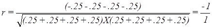
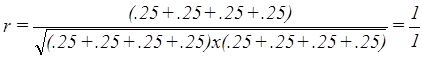
Recall that the formula for the
correlation is:
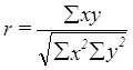
Note that all the little x scores
are either -.5 or +.5 indicating that the differences from the means are the
same for all cases. That is true for the
scores on TEST3 on the plot is considerably distant from the other tests. The scores are the differnence from their own
mean so that the distance between tests will be lost. Each score represents a difference from the
mean for that variable (in this example a test), however, the relative
distribution of the cases for that test will remain. Consequently, the correlation for TEST1 and
TEST2 is:
While the correlation between
TEST1 and TEST3 is:
And one more example of the
relationship between TEST1 and TEST4.
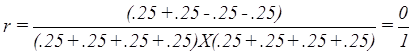
In this instance TEST1, TEST2,
and TEST3 are similar while TEST4 is different.
A look at cluster analysis tells
a different story.
|
File Name = crslis2.sps
|
|
get file =
'\proeval\CLSDAT1.sav'
/keep= PERs TEST1 TEST2 TEST3 TEST4.
COMPUTE dif12 = TEST1 ‑
TEST2.
COMPUTE dif13 = TEST1 ‑
TEST3.
COMPUTE dif14 = TEST1 ‑
TEST4.
compute dif12s=dif12*dif12.
compute dif13s=dif13*dif13.
compute dif14s=dif14*dif14.
LIST dif12 dif13 dif14 dif12s
dif13s dif14s.
|
|
CRSLIS2.SPS
|
|
DIF12 DIF13
DIF14 DIF12S DIF13S
DIF14S
‑1.00 ‑3.00 .00
1.00 9.00 .00
1.00
‑3.00 .00 1.00
9.00 .00
‑1.00 ‑3.00 ‑1.00 1.00
9.00 1.00
1.00
‑3.00 1.00 1.00
9.00 1.00
|
First note that in the absolute
differences between TEST1 and TEST2 (TEST1 minus TEST2) are all 1. However, half of them are in one direction
and the other half are in the opposite direction (note the minus signs). The differences square and summed equal
4. The differences between TEST1 and
TEST3 are all -3; the values squared and summed equal 36 indicating the most
dissimilarity. In the correlation
analysis these latter two variables had a perfect correlation. On the other hand tests 1 and 4 show the most
similarity where their squared differences cumulate to only 2. In the correlation analysis these two
variables had a correlation of zero indicating the relative positions to be the
most dissimilar. [The point of this is
for the investigator to decide what question is being asked.]
***
There is a difference in profile
but also a difference in that profiles can be opposite and still be a part of
the same factor (negatively related to the factor).
***
It might be useful at this point
to compare and contrast the various statistical procedures used in this
set. From a practical point of view
different techniques were selected and it might be useful to note why they were
selected for the various questions.
This chapter is provided to show
similarities and differences between the various statistical procedures.
This data set to be used is made
up of ratings of personality theories by 12 to 16 raters. The questionnaire used for these rating
follows:
Personality
Theory Rating Scale
Name:
_________________________________________
Date: ________________
Use the scale below to rate the
personality theory of ____________________________.
╔═══════════════════════════════════════════════════════════════════════════╗
║ None A Little Somewhat Quite a Bit A Lot ║
╟───────────────────────────────────────────────────────────────────────────╢
║ 0 1
2 3 4
5 6 7
8 ║
╚═══════════════════════════════════════════════════════════════════════════╝
╔══════════════════════╗
║LEAVE THE
QUESTION ║
║BLANK IF YOU
DON'T ║
║KNOW OR IF IT DOESN'T ║
║APPLY. ║
╚══════════════════════╝
ACCORDING
TO THIS THEORY:
_____
...motivation is based on drive reduction.
_____
...the person is an intentional (goal-oriented) being.
_____
...people are hedonistic.
_____
...cognition accounts for the actions of people.
_____
...values account for the actions of people.
_____
...people are actively involved in the development of their personality.
_____
...people's early experiences influence their personality.
_____
...the person imposes perception on the world.
_____
...the environment or learning accounts for the person's actions.
_____
...people are basically good.
_____
...heredity effects the person's actions.
_____
This theory stresses the individual's conscious view of the world.
_____
This theory stresses the individual's unconscious view of the world.
_____
This theory stresses the individual's social consciousness.
_____
This theory accounts for the individual's perception of reality.
_____
This theory has influenced psychology (clinical, research, literature).
_____
This theory focus on "the here and now", the past, or the
future.
(0 = past, 4 = here and now, 8 =
future)
_____
This theory is empirically based.
_____
This theory is parsimonious.
_____
This theory assumes that the individual has free choice.
_____
This theory employs a method of therapeutic intervention.
_____
This theory emphasizes psychopathology.
_____
I agree with this theory.
The names for the respective
items are as follows:
TDATE
THER
THID
CLUS
DRIVE
GOAL
HEDON
COG
VALUE
ACTIVE
EARLY
IMPOSE
LEARN
GOOD
HERED
CONSCI
UNCONS
SOCIAL
PERCEP
INFLU
TIME
DATA
PARSI
FREE
THERA
PATH
AGREE
The theorists rated were:
Freud Sigmund Freud
ADLER Alfred Adler
JUNG Carl Jung
ROGERS Carl Rogers
KELLY George Kelly
HORNEY Karen Horney
SULLIVI Harry Stack Sullivan
BANDURA Albert Bandura
CATTELL Raymond B. Cattell
MASLOW Abraham Maslow
BINSWAN Ludwig Binswanger
ERIKSON Erik Erikson
This data was part of a graduate
student class assignment for students taking a theories of personality
class. Each week the students read the
assignments and completed the questionnaire the day before the class
meeting. There were 17 students enrolled
in the class, however, not all students complete the forms each week and
consequently there is some missing data.
There were ___ completed forms.
In this first example the items
of the questionnaire are grouped using factor analysis. Recall that in this condition the items with
similar profiles will be grouped together (into factors); not necessarily the
items that are closest in distance (refer to the above discussion). The data is in a dBase IV file with 9
indicating that data was omitted. As can
be seen mostly defaults were used in the computer run (see Frame PERFAC5.SPS)
and a principle components extraction method was used and the rotation was
orthoginal. Using the eigenvalue of 1.00
is usually not considered the best method of deciding upon the number of
factors; however, both interpretation and the scree method seemed also to
indicate 5 factors.
|
File Name = perfac5.sps
|
|
get file=
'\proeval\perall4.sav'/keep=
tDATE THER
THID CLUS DRIVE
GOAL HEDON COG
VALUE ACTIVE EARLY
IMPOSE LEARN
GOOD HERED CONSCI
UNCONS SOCIAL PERCEP
INFLU TIME
DATA PARSI FREE
THERA PATH AGREE .
missing values drive to agree
(9).
fac var= drive to agree
/missing=pairwise
/plot=eigen
/criteria=factors(5)
/rotate.
|
┌────────────────────────────────────────────────────────────────────────────┐
│
PERFAC5.LIS
│
├────────────────────────────────────────────────────────────────────────────┤
│Final Statistics: │
│
│
│Variable Communality *
Factor Eigenvalue Pct of Var
Cum Pct │
│ * │
│DRIVE .54238 *
1 6.98937 30.4 30.4 │
│GOAL .50485 *
2 2.15730 9.4 39.8 │
│HEDON .54444 *
3 1.72904 7.5 47.3 │
│COG .56063 *
4 1.47348 6.4 53.7 │
│VALUE .66169 *
5 1.32890 5.8 59.5 │
│ACTIVE .70979 *
│
│EARLY .58670 *
│
│IMPOSE .64661 *
│
│LEARN .58716 *
│
│GOOD .51995
*
│
│HERED .58137 *
│
│CONSCI .64024 *
│
│UNCONS .68112 *
│
│SOCIAL .61566 *
│
│PERCEP .61891 *
│
│INFLU .59501 * │
│TIME .58200 *
│
│DATA .56921 *
│
│PARSI .60125 * │
│FREE .61128 *
│
│THERA .64608 *
│
│PATH .52881 *
│
│AGREE .54294
*
│
│
│
│Rotated Factor
Matrix:
│
│ │
│ FACTOR 1
FACTOR 2 FACTOR
3 FACTOR 4
FACTOR 5 │
│
│
│DRIVE ‑.67035** ‑.10424 ‑.12588 ‑.21679 .13893
│
│GOAL .44300 .44580* .16215 .17344 .23128
│
│HEDON ‑.72226** ‑.01600 .14498 .01324 .03653
│
│COG .50422* .28914 .40228 .23887 ‑.06251 │
│VALUE .15529 .79294** ‑.08091 ‑.04701 .00768
│
│ACTIVE .58000** .41073 .21364 .39876 ‑.00630 │
│EARLY ‑.69231** .27344 ‑.13863 .07009 .09220
│
│IMPOSE .22239
.23344 ‑.10607 .72878** .01706
│
│LEARN .02767 .45879 .49137* .21355 ‑.29809 │
│GOOD .57563** .41920 .00750 ‑.00350 .11316
│
│HERED .10169 .28821 ‑.34325 ‑.60077** ‑.09606 │
│CONSCI .55734** .40202 .29750 .26467 ‑.09712 │
│UNCONS ‑.48833* ‑.19803 ‑.48205 ‑.38498 .15119
│
│SOCIAL ‑.05895 .71266** .26140 .18852 .02080
│
│PERCEP .29944 .16227 ‑.10921 .69839** .05684
│
│INFLU ‑.10405 .01029 .21463 ‑.17453 .71242**│
│TIME .72841** .04942 .11085 .18045 ‑.06419 │
│DATA .29151 .04499 .63344** ‑.20723 .19498
│
│PARSI .05321 .06473 .76207** .00803 .11581
│
│FREE .51295* .32588 .28510 .39853 .04315
│
│THERA ‑.13541 ‑.11914 ‑.26013 .24730 .69622**│
│PATH ‑.51195* ‑.08011 ‑.40072 ‑.11859 .29269
│
│AGREE ‑.01068 .34696 .25436 .21198 .55930**│
└────────────────────────────────────────────────────────────────────────────┘
We were somewhat arbitrary in
selecting 5 factors in this solution so that it would match with the five
cluster solution in the cluster analysis solution that follows. It should be noted that one should not be so
casual in determining the number of factors in a solution; the reader is
referred to chapter __ when testing for the number of factors. In developing theory the researcher may do
that in an armchair fashion, reviewing the literature or with exploratory
factor analysis. The major purpose here
to compare factor analysis with cluster analysis so that the number of factors
is done with that purpose in mind.
The factors in Figure __ are
presented in two ways: (1) the criterion of .60 is used to determine whether a
variable loads on a factor, (2) if a variable does not load on any factor then
it is placed on the factor with the highest loading.
Factor I
DRIVE -.67
HEDON -.72
EARLY -.69
TIME .73
---------
GOAL .44
COG .50
ACTIVE .58
GOOD .58
CONSCI .56
UNCONS -.49
FREE .51
PATH -.51
Factor II
VALUE .79
SOCIAL .71
-----------
GOAL .45
Factor III
DATA .63
PARSI .76
----------
LEARN .49
Factor IV
IMPOSE .73
HERED -.60
PERCEP .70
Factor V
INFLU .71
THERA .70
AGREE .56
The next example shows how
cluster analysis can be used to group the same set of data. The data needs to be conditioned before the
cluster analysis can be run. The means
are computed within each theorist for each item. For example, the first item DRIVE for all
respondents to Freud were summed and divided by the number of respondents (the
number was also rounded to the nearest integer to keep it on the same
scale). The matrix was then transposed
because the computer program requires that format for this problem. This data is presented in the frame THER11.sav.
|
ITEM
|
FREUD
|
ADLER
|
JUNG
|
ROGERS
|
KELLY
|
HORNEY
|
SULLIVA
|
BANDURA
|
CATTELL
|
MASLOW
|
BINSWAN
|
ERIKSON
|
|
DRIVE
|
8
|
2
|
3
|
2
|
2
|
3
|
4
|
1
|
3
|
4
|
2
|
4
|
|
GOAL
|
4
|
7
|
5
|
7
|
7
|
5
|
5
|
6
|
5
|
7
|
5
|
6
|
|
HEDON
|
7
|
3
|
2
|
2
|
2
|
4
|
4
|
2
|
3
|
4
|
3
|
3
|
|
COG
|
3
|
6
|
4
|
6
|
7
|
4
|
5
|
7
|
5
|
6
|
6
|
6
|
|
VALUE
|
4
|
6
|
5
|
6
|
4
|
4
|
5
|
5
|
4
|
6
|
6
|
6
|
|
ACTIVE
|
2
|
7
|
5
|
7
|
7
|
5
|
5
|
6
|
5
|
6
|
7
|
6
|
|
EARLY
|
8
|
7
|
4
|
5
|
4
|
6
|
6
|
5
|
4
|
5
|
4
|
7
|
|
IMPOSE
|
4
|
6
|
4
|
7
|
7
|
5
|
6
|
5
|
5
|
6
|
7
|
6
|
|
LEARN
|
3
|
6
|
3
|
5
|
5
|
6
|
6
|
7
|
6
|
5
|
5
|
6
|
|
GOOD
|
2
|
5
|
5
|
8
|
5
|
4
|
4
|
5
|
4
|
6
|
4
|
6
|
|
HERED
|
3
|
4
|
5
|
4
|
2
|
3
|
3
|
2
|
5
|
4
|
3
|
4
|
|
CONSCI
|
2
|
6
|
5
|
6
|
6
|
4
|
5
|
6
|
5
|
6
|
6
|
6
|
|
UNCONS
|
8
|
2
|
7
|
3
|
2
|
6
|
4
|
2
|
4
|
3
|
2
|
5
|
|
SOCIAL
|
4
|
7
|
3
|
6
|
5
|
5
|
6
|
6
|
5
|
5
|
5
|
6
|
|
PERCEP
|
5
|
6
|
5
|
7
|
7
|
5
|
6
|
6
|
5
|
6
|
7
|
5
|
|
INFLU
|
8
|
5
|
5
|
7
|
4
|
3
|
5
|
6
|
5
|
6
|
4
|
5
|
|
TIME
|
0
|
5
|
5
|
4
|
5
|
3
|
4
|
4
|
5
|
5
|
5
|
3
|
|
DATA
|
3
|
3
|
2
|
4
|
4
|
2
|
4
|
6
|
6
|
3
|
2
|
4
|
|
PARSI
|
4
|
5
|
3
|
5
|
6
|
4
|
4
|
5
|
5
|
5
|
3
|
5
|
|
FREE
|
2
|
5
|
3
|
7
|
7
|
5
|
4
|
6
|
4
|
6
|
7
|
5
|
|
THERA
|
7
|
5
|
6
|
7
|
6
|
5
|
6
|
5
|
3
|
3
|
5
|
5
|
|
PATH
|
7
|
3
|
5
|
3
|
3
|
6
|
5
|
3
|
4
|
3
|
4
|
4
|
|
AGREE
|
5
|
5
|
4
|
5
|
5
|
5
|
5
|
5
|
4
|
5
|
4
|
5
|
|
File
Name = percls3.sps
|
|
get
file = '\proeval\ther11.sav'/keep=
ITEM FREUD
ADLER JUNG ROGERS KELLY
HORNEY
SULLIVA BANDURA
CATTELL MASLOW BINSWAN
ERIKSON.
cluster
freud to erikson
/id=item
/print=distance
/print=schedule cluster(5)
/plot=dendrogram hicicle.
|
* * * * * * H I E R A R C H I C A L C L U S T E R A N A L Y S I S * * * * * *
Dendrogram using Average Linkage (Between
Groups)
Rescaled Distance
Cluster Combine
C
A S E 0 5 10 15 20 25
Label Num +---------+---------+---------+---------+---------+
IMPOSE 8 òûòø
PERCEP 15 ò÷ ó
GOAL 2 òòòüòø
COG 4 òø ó ó
CONSCI 12 òôò÷ ùòòòø
ACTIVE 6 ò÷ ó ùòø
FREE 20 òòòòò÷ ó ó
VALUE 5 òòòòòòòûò÷ ùòòòòòòòòòø
GOOD 10 òòòòòòò÷ ó
ó
LEARN 9
òûòòòòòø ó ó
SOCIAL 14 ò÷ ùòòò÷ ùòòòòòòòòòòòø
PARSI 19 òûòòòòò÷ ó ó
AGREE 23 ò÷ ó ó
INFLU 16 òòòòòòòòòòòòòø ó
ùòòòòòòòòòòòòòòòø
THERA 21 òòòòòòòòòòòòòüòòòòòòò÷ ó ó
EARLY 7 òòòòòòòòòòòòò÷ ó ó
HERED 11 òòòòòòòòòòòòòòòûòòòø ó ó
TIME 17 òòòòòòòòòòòòòòò÷ ùòòòòòòòòòòòòò÷ ó
DATA 18 òòòòòòòòòòòòòòòòòòò÷ ó
DRIVE 1 òûòòòòòòòòòòòòòø ó
HEDON 3 ò÷
ùòòòòòòòòòòòòòòòòòòòòòòòòòòòòòòòòò÷
UNCONS 13 òòòòòûòòòòòòòòò÷
PATH 22 òòòòò÷
If
five factors are chosen (to be comparable to the 5 factor solution above) there
are as follows:
Cluster
1
IMPOSE
PERCEP
GOAL
COG
CONSCI
ACTIVE
FREE
VALUE
GOOD
LEARN
SOCIAL
PARSI
AGREE
Cluster
2
INFLU
THERA
EARLY
Cluster
3
HERED
TIME
DATA
Cluster
4
DATA
Cluster
5
DRIVE
HEDON
UNCONS
PATH
The
first question is whether there is a difference between the factor analysis
solution and the cluster analysis solution?
There is not a test of significance that can be run [or would Chi Square
be appropriate? there is the problem of what is a match is it two or more
variables in the same group; cluseter or factor or must all overlap] so it
mostly a matter determining whether appears that the solution are the same or
different. If one chooses to the
criteria of two or more variables in the same group then it does not look too
bad. Four variables from cluster 1 can
be found in factor 1; 3 variables from cluster 1 can be found in factor 2 (all
of factor 2); 2 variables in cluster 2 can be found in factor 5; and 4
variables in cluster 5 can be found in factor 1. That is 16 variables that overlap and 8
variables that do not [something wrong with this count]. That does give some indication that there is
some fit of the two methods. However,
cluster 3 does not have any variables that are shared in any of the factors and
factor 4 does not have any variables that are shared in any of the clusters. Further, cluster 1 and factor 1 are
fragmented across the two methods.
Finally, if one tries to develop a taxonomy from the two methods it
would seem to be different for the two methods.
[COMMENT1]The graph
with the 4 people is clsdat3.cdr