More Principles Underlying the General Linear
Model
There are two analyses
presented in this chapter -- the formulae and computations are the same as the
analysis in chapter 2. More data has been added to make it a more realistic
problem. The second analysis is designed to show the similarity between
analysis of regression and analysis of variance.
This chapter builds on
chapter 2 and if there are points that you don't understand because of
complexity of numbers it might be useful to refer to the more simplified set in
chapter 2. A correlation between continuous variables is presented as the first
example then a correlation between a continuous variable and a dichotomous
variable will be presented. The similarities between this correlation and an analysis
of variance will be shown.
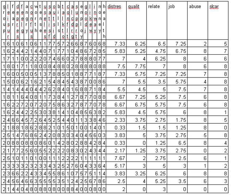
The sample data was
selected from a larger set that was administered to 5 different groups
including psychiatric inpatients and professional staff that worked with
psychiatric inpatients.
The problems throughout this chapter use sample
data from the preceding questionnaire. It should be recognized that is selected
data -- that is incomplete and selected for the purpose of this example. At the
same time is does represent results from a larger study. It is somewhat exaggerated
here in that the two samples are: (1) patients at the time of admission to an
inpatient hospital and (2) professional staff members. The data is randomly
selected from those groups excluding subjects who had missing data. Only 20
cases were selected (10 from each group) so that the mathematical calculations
can be followed.
Click here for a presentation by Trochim. If anyone finds a better description please
post it.
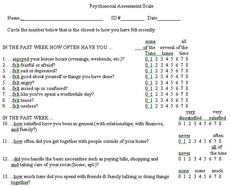
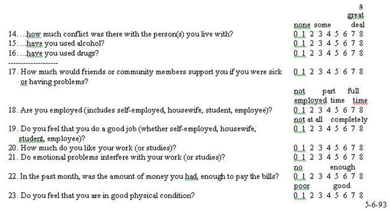
The Psychosocial Assessment Scale follows:
A Numerical Example
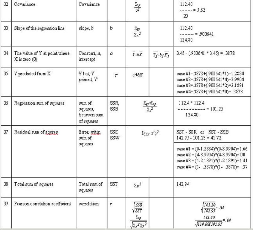
We are striving to understand the
formula
![]()
most of the general linear model.
Click
here to a result from multiple regression.
The complete General Linear Model also contains
an error element
Y'=a + bX + e.
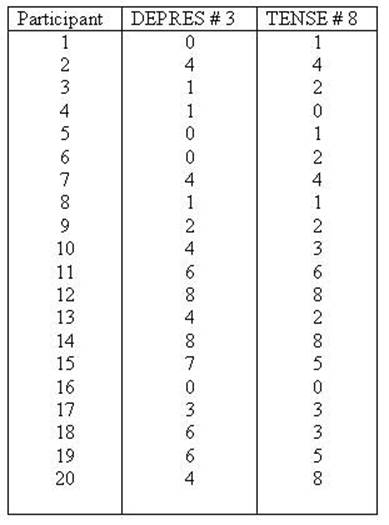
This example deals with
only items # 3 and # 8 of the questionnaire. Those questions were "In the
past week how often have you felt sad or depressed?" and "In the past
week how often have you felt tense?" and are labeled as DEPRES and TENSE
respectively. A discussion of the correlation between
responses to these two items (items 3 and 8 on the questionnaire) follows.
We will now present this data in the same way as
the more limited data was presented in chapter 2. So that all of the formulae
are the same as those presented in chapter 2 you're not learning a new set.
This is a more alive example and goes through the same process as in the
previous chapter. The variable TENSE is labeled as the X variable (predictor or
independent variable) and DEPRES as the Y variable (criterion or dependent
variable). First the data will be presented and the SPSS syntax files to
compute it will be given.
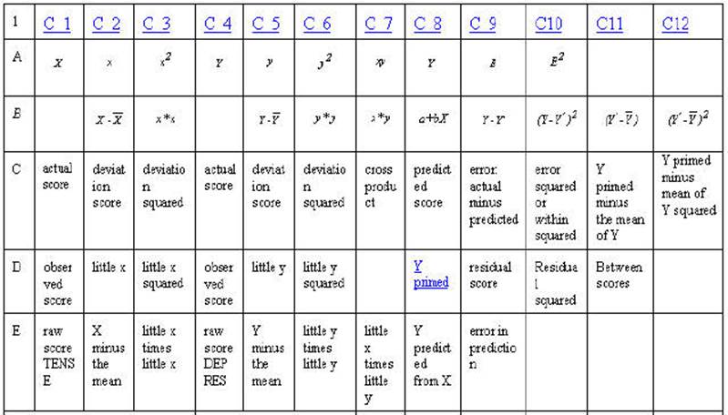
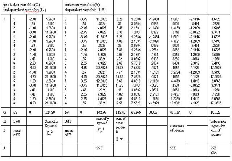
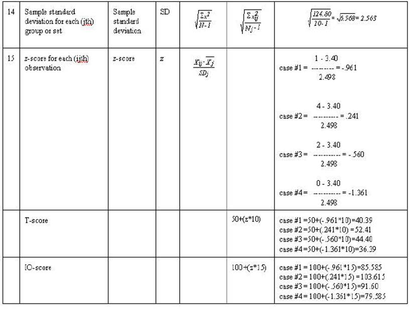
Table 2-3. Rows A through F are either
mathematical notation or verbal description of mathematical calculations of the
numbers in the column. Rows 1 through 20 are associated numbers involved the
calculation. Row G is the sum of the numbers in the column while row H is the
mean for the column. Row I is the usual verbal description of the sum in the
column and row J is an abbreviation of that description.
In the example below when there are scores for
all 20 cases are individually computed only the first 4 will be given (this
occurs with observation, little x, Y' and SSE).

The correlation and
regression can be shown graphically in terms of the General Linear
Model to develop understanding.
Graphic Representation of Sums of Squares
Regression
![]()
This
is presented in same manner as the Graphic Representation of the Sum of Squares
t-test
The
following scatterplot was generated from data taken from the Psychosocial
Assessment Scale
The correlation and
regression can be shown graphically to develop understanding.
Click here
to see how these scatterplots are generated
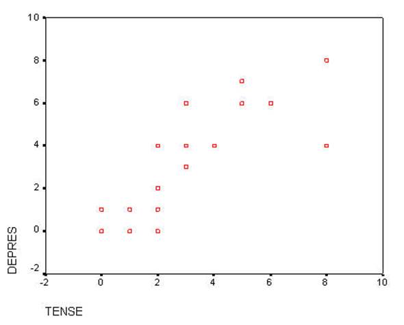
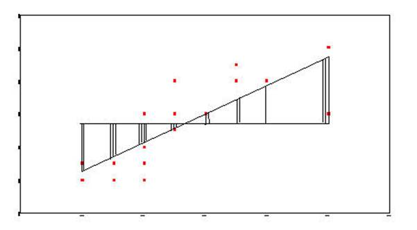
This scattergram
represents all of the respondents on the items of TENSE and DEPRES. People who
responded with smaller numbers to the item TENSE also responded with smaller
numbers to DEPRES. At the same time people who responded with larger numbers to
TENSE also responded with larger numbers to DEPRES. This plot represents two
variables DEPRES and TENSE. Person 16 answered both questions 0. Persons 12 and
14 answered both questions 8. Person 6 responded 2 to TENSE and a 0 to DEPRES.
You might want to identify some more of the cases to convince yourself of the
relationship of the data to the plot
The next three plots all have the same data as the previous but have
modifications drawn to show characteristics of the correlation or regression.
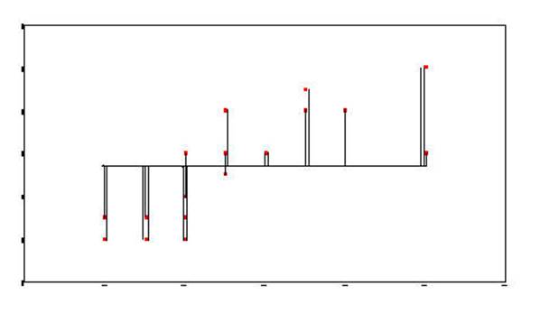
The next plot shows the sum of squares due to error or residual. It is the
error in predicting Y from X. TENSE is the X variable and DEPRES is the Y
variable.
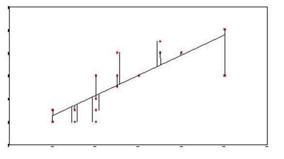
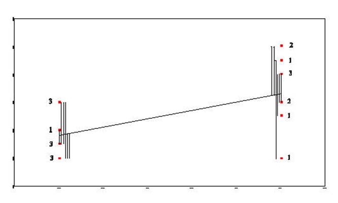
Sum-of-Squares-Residual (or
Sum-of-Squares-Error) are generated by taking the
distance from each data point and the regression line, squaring it, and adding
all of the squared distances together.
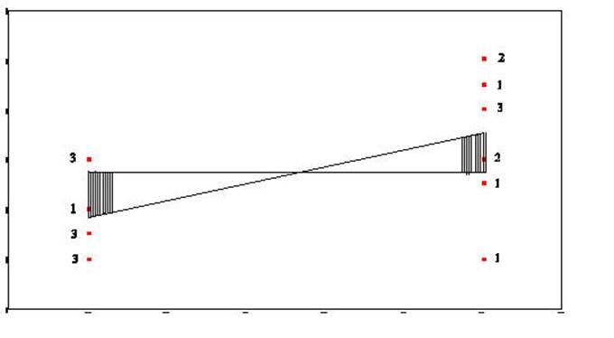
Sum-of-Squares-Regression (or Sum-of-Squres-Between) is generated by taking the distance from
the mean of Y and the regression line and squaring it. This is done for
each data point. Each of these squared distances is added together to
become the Sum-of-Squares-Regression (Sum-of-Squares-Between).
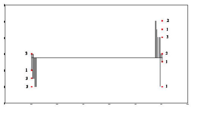
The Total-Sum-of-Squares is generated by
squaring the distance from the mean of Y and each data point and then summing
the squared results.
Click
here for the numeric process of obtaining SSE
Graphic Representation of Sums of Squares ANOVA
This is presented in same manner as the Graphic
Representation of the Sum of Squares Regression
The t-test can be
shown graphically in terms of the General Linear Model to develop
understanding.
The
following scatterplot was generated from data taken from the Psychosocial
Assessment Scale
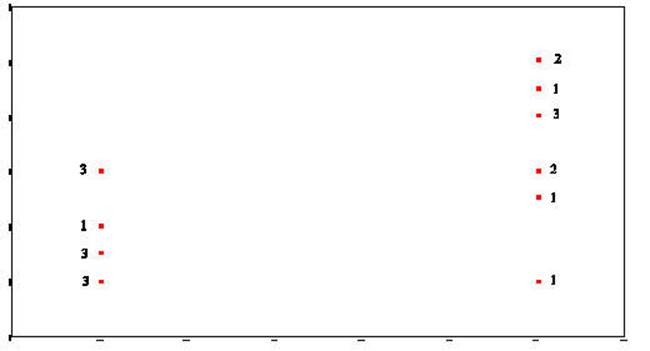
This plot represents two variables DEPRES and
GROUP. There were three people in GROUP # 1 who answered 0 to the question of
"sad or depressed." If you look back at the raw data you will that
was participants 1, 5, and 6. There was one person in GROUP # 2 that answered
the question as 0. In looking at the raw data you will see that it was person #
16. There were two people in GROUP # 2 that answered the question as 8. There
were person number # 12 and person # 14. This scattergram
represents all the people of both groups. Once again the scattergram
represents a relationship. The smaller going with the small
and the large with the large. People in GROUP # 1 gave responses which
were smaller and people in GROUP # 2 (2 is larger than one) gave responses
which were larger than those in GROUP # 1.
The two variables DEPRES and GROUP follow:
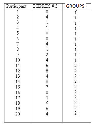
Group
#1 Group
# 2
![]()
Sum-of-Squares-Residual (or
Sum-of-Squares-Error) are generated by taking the
distance from each data point and the regression line, squaring it, and adding
all of the squared distances together.
Sum-of-Squares-Regression (or Sum-of-Squres-Between) is generated by taking the distance from
the mean of Y and the regression line and squaring it. This is done for
each data point. Each of these squared distances is added together to
become the Sum-of-Squares-Regression (Sum-of-Squares-Between).
The Total-Sum-of-Squares is generated by
squaring the distance from the mean of Y and each data point and then summing
the squared results.